legislatoR
legislatoR is a package for the software environment R that facilitates access to the Comparative Legislators Database (CLD). The package is available through CRAN and GitHub. To install the package from CRAN, type:
install.packages("legislatoR")
You can also download the development version directly from Github:
#install.packages("devtools")
devtools::install_github("saschagobel/legislatoR")
Usage
A working Internet connection is required to access the CLD in R. This is because the data are stored online and not installed together with the package. The package provides table-specific function calls. These functions are named after the respective table and preceded by legislatoR::get_. To fetch the Core table, use the legislatoR::get_core() function, for the Political table, use the legislatoR::get_political() function. Call the package help file via ?legislatoR() to get an overview of all function calls. Tables are legislature-specific, so a letter country code must be passed as an argument to the function. Here is a breakdown of all country codes. You can also call the legislatoR::cld_content() function to get an overview of the CLD's scope and valid country codes.
| Legislature | Code | Legislature | Code | Legislature | Code |
|---|---|---|---|---|---|
| Austrian Nationalrat | aut |
German Bundestag | deu |
UK House of Commons | gbr |
| Canadian House of Commons | can |
Irish Dail | irl |
United States Congress | usa_house/usa_senate |
| Czech Poslanecka Snemovna | cze |
Scottish Parliament | sco |
||
| French Assemblée | fra |
Spanish Congreso | esp |
Working with the legislatoR package in R
The legislatoR package provides an easy-to-use interface to the CLD in R. This brief tutorial will present two use-cases to illustrate how to engage the different tables of the database to extract information for analyses. To be precise, we will:
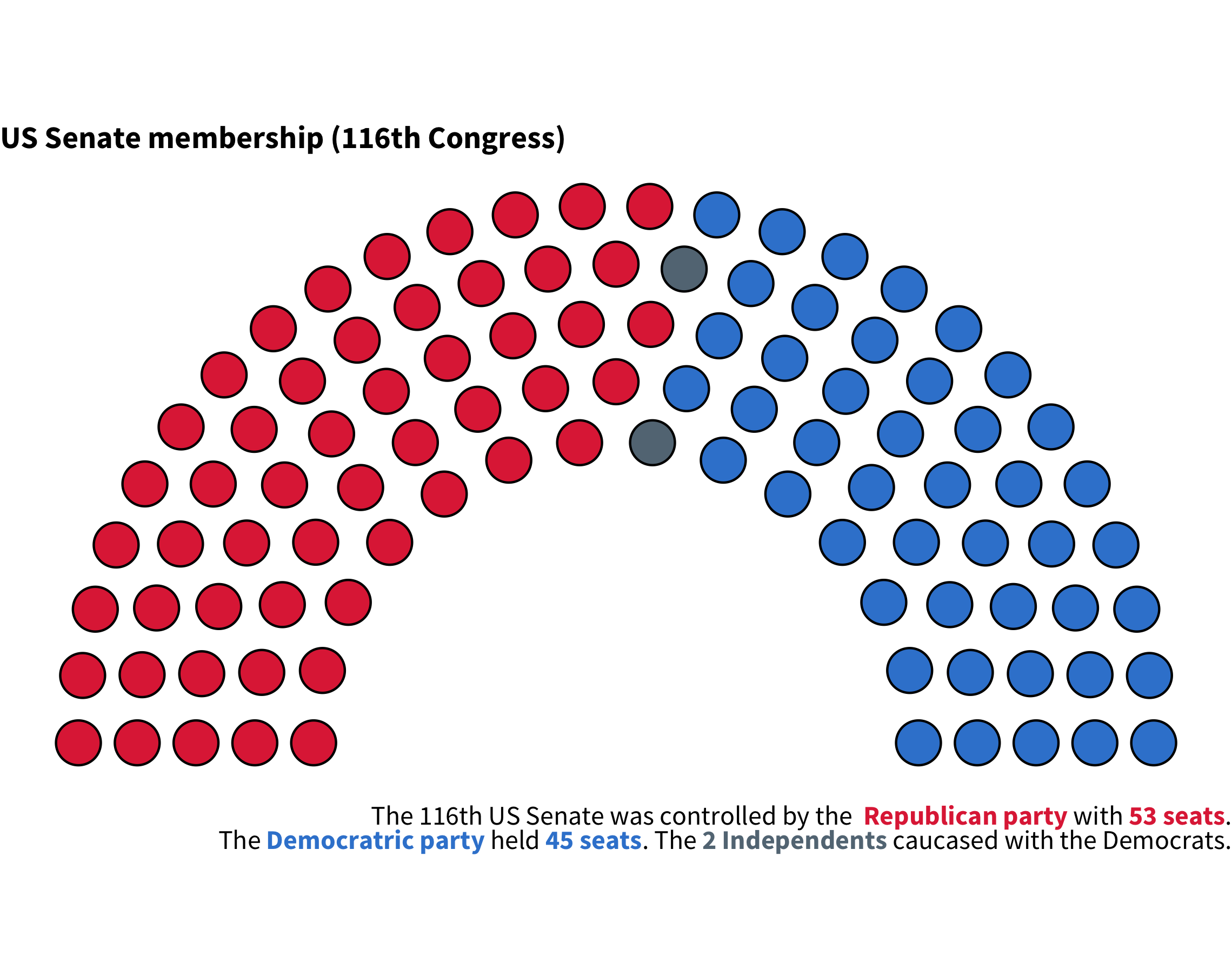
- explore the distribution of seats in the U.S. Senate during the 116th United States Congress (Jan 2019 - Jan 2021)
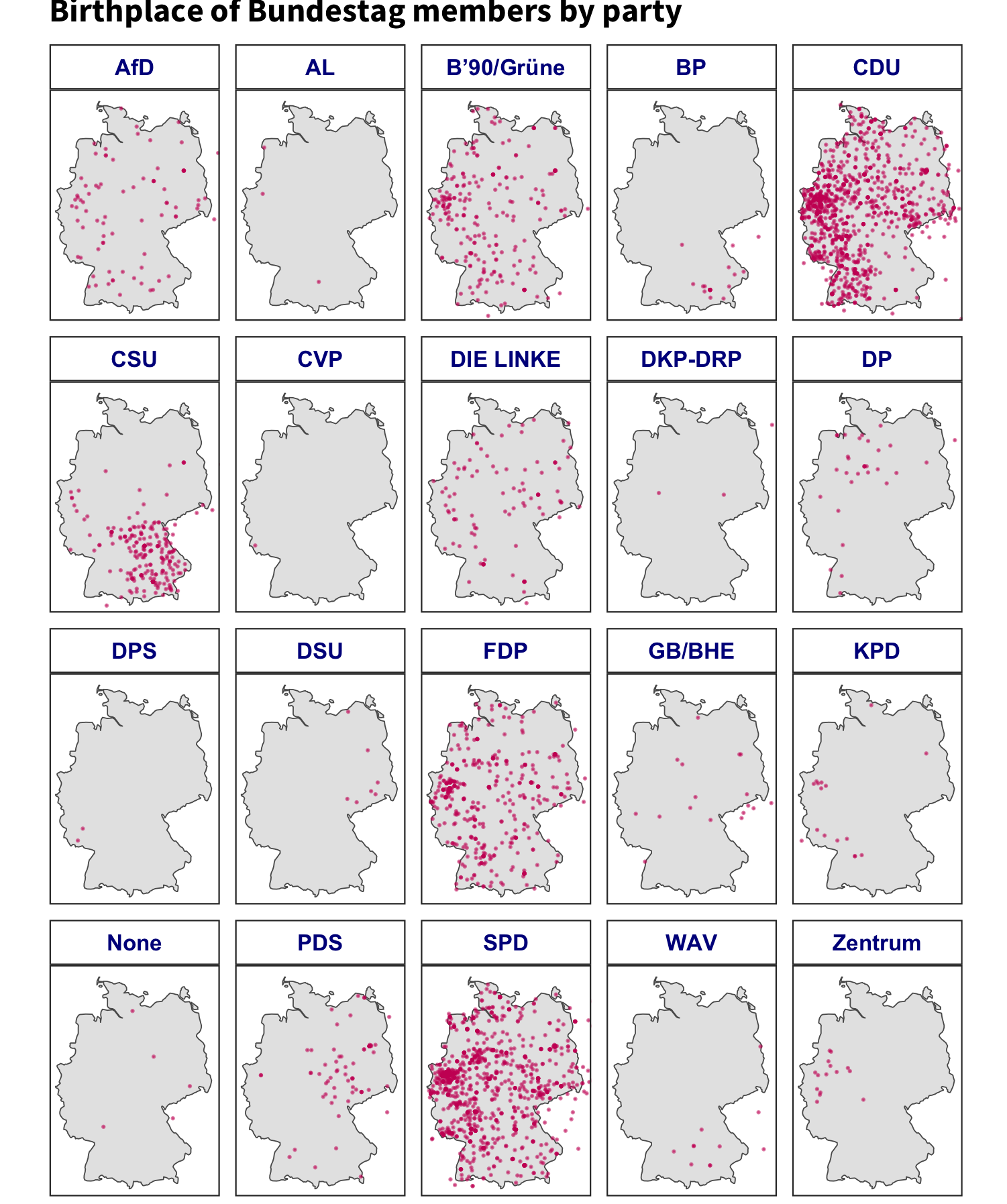
- map the birthplaces of all the members of the Bundestag by political party
# load the libraries
library(legislatoR)
library(dplyr) #data manipulation
library(ggplot2) #data visualization
library(ggtext) #text aesthetics in ggplot2
library(ggpol) #geom_parliament() (parliament plots)
library(sf) #spatial vector encodings in R
library(rnaturalearth) #natural earth map data
library(rnaturalearthdata) #natural earth map data

set.seed(1310) # to get consistent results from randomization
The U.S. Senate during the 116th United States Congress
The Core table is at the center of the database structure. This table contains basic demographic information about the legislators, in addition to the joining keys: Wikipedia page ID (pageid) and the Wikidata ID (wikidataid). These data can be retrieved through the get_core() call function. The call functions take the legislature code as an argument (i.e., get_*(legislature="code")). Each table can be called independently based on the use-case and can be linked through one of the joining keys.
# load US Senate core
legislatoR::get_core(legislature = "usa_senate") %>%
dplyr::sample_n(10) #get ten random entries
In this case, we will employ Political table to derive the counts of the seats each party held:
# load US Senate political table for the 116th Congress
us_senate_political <- legislatoR::get_political(legislature = "usa_senate") %>%
  dplyr::filter(session == 116) #filter only legislators from the 116th Congress

dplyr::sample_n(us_senate_political, 10) #print ten random entries
You can employ dplyr verbs to extract the seat counts per party and generate a visual illustration of the distribution:
# get the seat counts per party for parliament plot
us_senate_counts <- us_senate_political %>%
  dplyr::group_by(party) %>% #nest at party
  dplyr::summarize(seats = n()) %>% #generate counts
  dplyr::mutate(colors = dplyr::case_when(party == "D" ~ "#3885D3",
  party == "R" ~ "#E02E44",
  party == "Independent" ~ "#637684")) #assign party colors for visualization

us_senate_counts
We can use the us_senate_counts data frame as the input for our plot:
# a caption with some md formating
caption_plot <- paste0("The 116th US Senate was controlled by the <b style='color:#E02E44'> Republican party</b> with <b style='color:#E02E44'>",
us_senate_counts$seats[us_senate_counts$party == "R"], # Number of Republican seats
" seats</b>.<br>The <b style='color:#3885D3'>Democratric party</b> held <b style='color:#3885D3'>",
us_senate_counts$seats[us_senate_counts$party == "D"], # Number of Democrat seats
" seats</b>. The <b style='color:#637684'>",
us_senate_counts$seats[us_senate_counts$party == "Independent"], # Number of Independent seats
" Independents </b>caucased with the Democrats."
)
# plot parliament seats
ggplot(us_senate_counts) +
ggpol::geom_parliament(aes(seats = seats, fill = party), color = "black") +
scale_fill_manual(values = us_senate_counts$colors, labels = us_senate_counts$party) +
coord_fixed() +
labs(title = "<b>US Senate membership (116th Congress)</b>",
caption = caption_plot) +
theme_void() +
theme(legend.position = "none",
plot.title = ggtext::element_markdown(),
plot.caption = ggtext::element_markdown())
The birthplaces of German parlimentarians
In most instances, you will need to link information from different tables in the database. For instance, in this case we need the parliamentarians' birthplace coordinates and their political party. These two data points are in the Core and Political tables. One easy way to link the tables is by employing dplyr joins.
# assign Political and Core tables to the environment
deu_politicians <- dplyr::left_join(x = legislatoR::get_political(legislature = "deu"),
                                    y = legislatoR::get_core(legislature = "deu"),
                                    by = "pageid") #these two tables can be joined through their Wikipedia page ID

head(deu_politicians) #print first couple observations
The deu_politicians data frame contains all the information from the two tables. We can use these data to extract the latitudes and longitudes of the legislators' birthplace for a map.
# extract birthplace latitudes and longitudes with regular expressions
deu_birthplace_map_df <- deu_politicians %>%
  dplyr::distinct(wikidataid, .keep_all = T) %>% # keep unique entries of legislators
  dplyr::mutate(lat = stringr::str_extract(birthplace, "[-[:digit:]]{1,4}\\.[:digit:]+") %>% as.numeric(),
                lon = stringr::str_extract(birthplace, "[-[:digit:]]{1,4}\\.[:digit:]+$") %>% as.numeric())

# define German boundaries
lat1 <- 47; lat2 <- 55.5 ; lon1 <- 5.5; lon2 <- 15.5

germany_sf <- rnaturalearth::ne_countries(scale = "medium", returnclass = "sf", country = "Germany") #get spatial encodings for Germany

ggplot(germany_sf) +
  geom_sf(size = 1) +
  geom_point(data = deu_birthplace_map_df, aes(x = lon, y = lat), size = .25,
  shape = 20, color = "#cc0065", alpha = 0.5) +
  theme_bw() +
  facet_wrap(~party) +
  coord_sf(xlim = c(lon1, lon2), ylim = c(lat1, lat2), expand = FALSE) +
  labs(title = "<b>Birthplace of Bundestag members<b>")+
  theme(plot.margin=grid::unit(c(0,0,0,0), "mm"),
  axis.title = element_blank(),
  axis.ticks = element_blank(),
  axis.text=element_blank(),
  panel.grid.major = element_blank(),
  panel.grid.minor = element_blank(),
  legend.position = "none", text = element_text(size=10),
  panel.grid.minor.y =  element_blank(),
  strip.background = element_rect(fill="white"),
  strip.text.x = element_text(color = "darkblue", face = "bold"),
  plot.title = ggtext::element_markdown(family = "Source Sans Pro"))